Image Segmentation Guide

Image segmentation assigns a class to every pixel. AnyLearning calls the task Image Segmentation; it is commonly called semantic segmentation elsewhere. Pixels outside your foreground classes become the implicit background class. This guide uses electron-microscopy particles as a compact real example.

Step 1: Create a Project

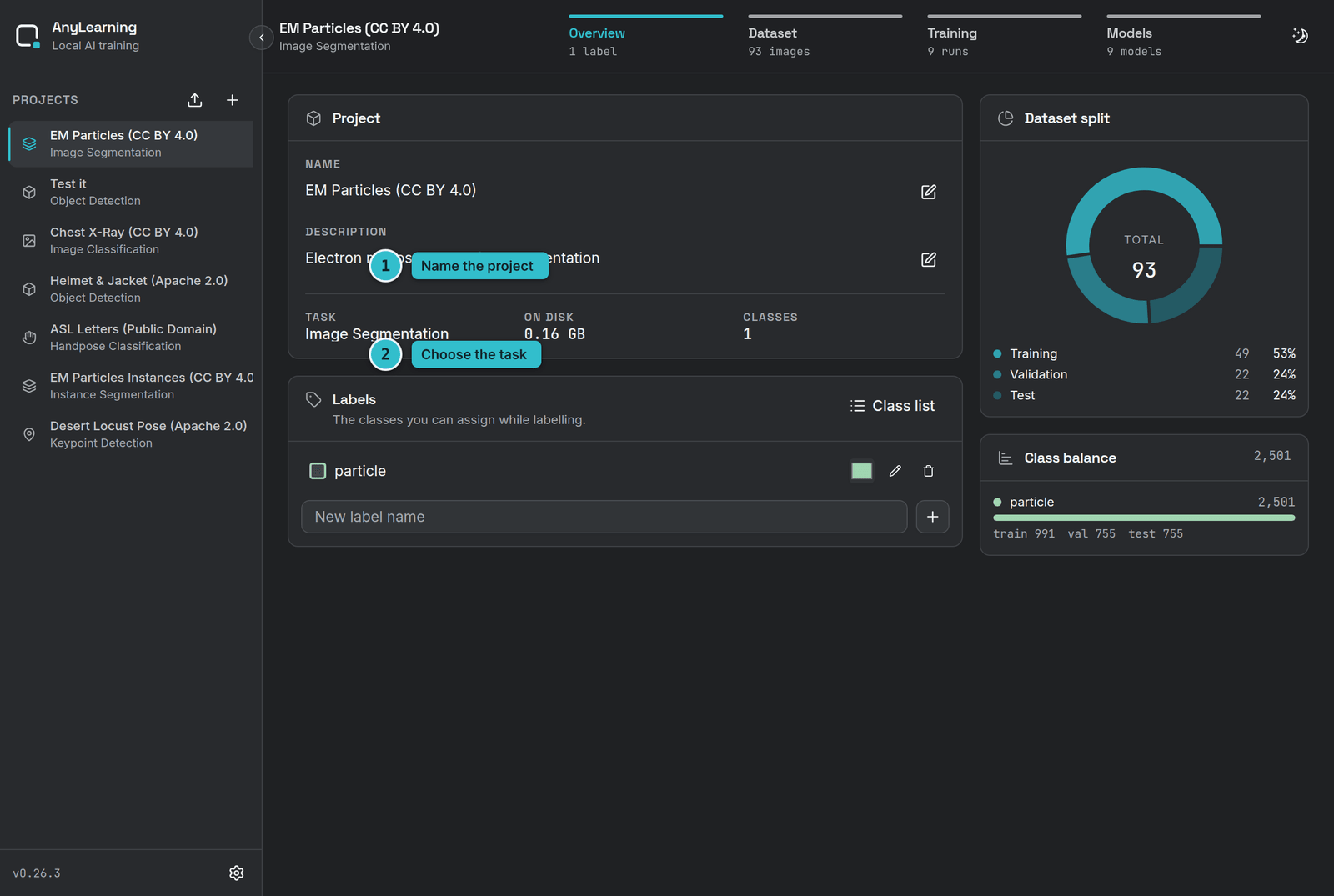
First, create a new project specifically for image segmentation:

Click Create project
Pick Image Segmentation as the task
Provide a meaningful project name and description

Project creation

Step 2: Data Preparation

2.1. Create the Label Set

The label set defines all possible pixel classes that your model will learn to segment. For example, in a microscopy particle segmentation project, your label might be particle.

To create your label set:

Navigate to the Overview tab
Enter each class name individually in the input field
Click + after each class name
Ensure class names are descriptive and consistent

Create label

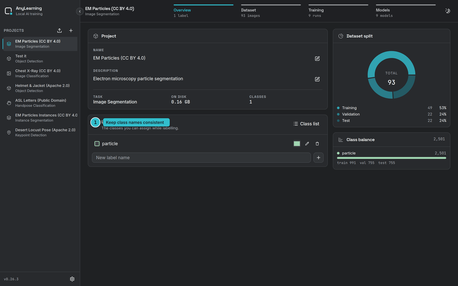
If an imported archive already contains annotations, AnyLearning can create the label set from it. You do not need to enter the classes twice.

2.2. Upload the Datasets

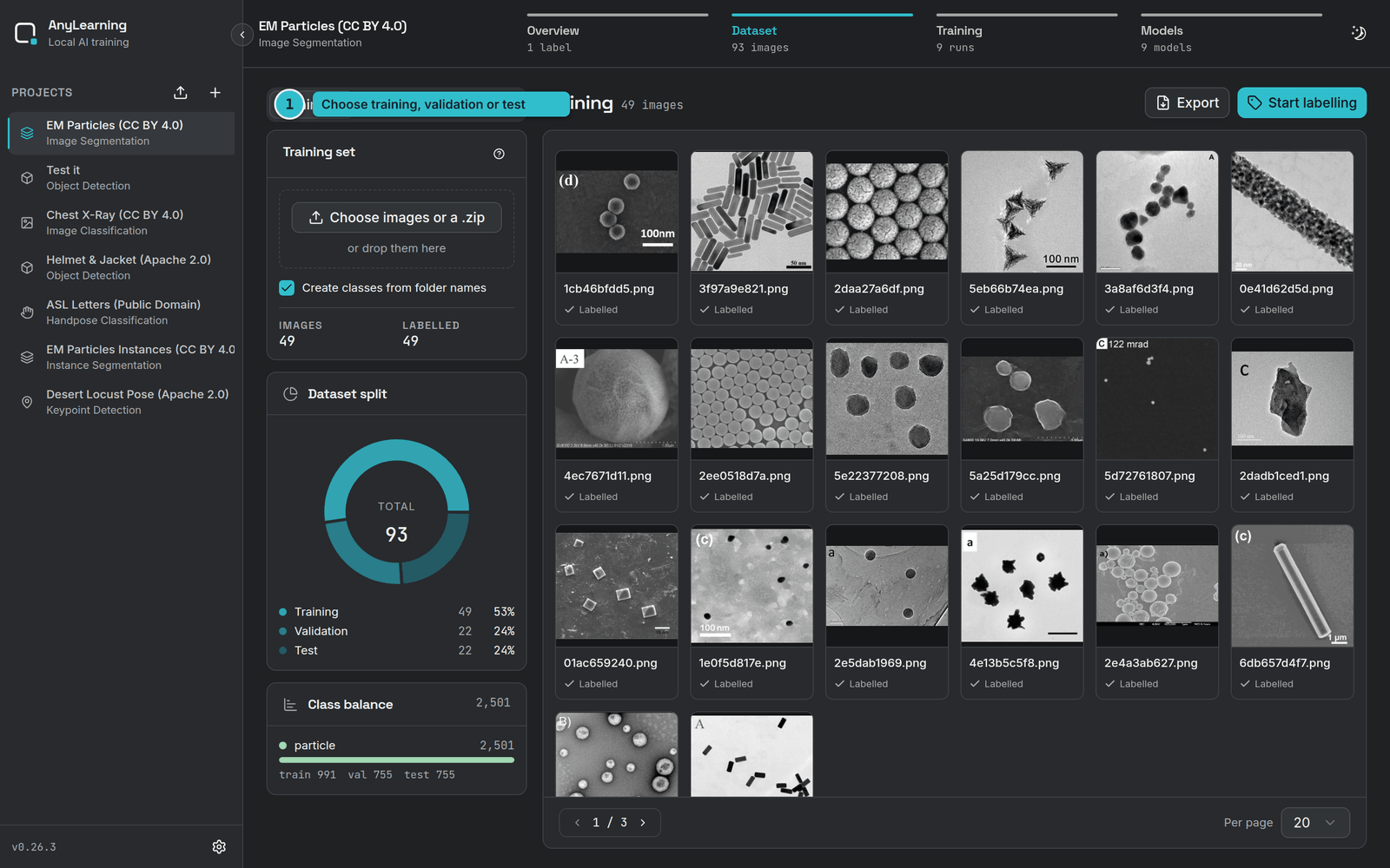
Go to the Dataset tab to manage your datasets.

For effective model training, split your data into three sets:

Training set: The largest portion (typically 70-80%) used to train the model
Validation set: A smaller portion (typically 10-15%) used to tune hyperparameters and prevent overfitting
Test set: The remaining portion (typically 10-15%) used to evaluate the final model performance

Upload Process:

Go to the Dataset tab and choose the Training, Validation or Test set.
Click Choose images or a .zip, or drop files straight onto the panel. Several images at once is fine, and so is one .zip per split.
If your images are already annotated, upload the archive as it is: COCO, YOLO, LabelMe and AnyLabeling are all read, and the annotations come in with the images. Ticking Create classes from folder names takes the class list from the archive rather than needing step 2.1 first.
Wait for the upload to finish. The image and label counts under the panel update as it goes.

Trial dataset: Download the prepared electron-microscopy splits from Hugging Face (opens in a new tab).

Important: Ensure masks are correctly labeled, with each pixel corresponding to a class in your label set.

Dataset upload

(1) Labelme json annotation format example:

{
  "version": "4.2.10",
  "flags": {},
  "shapes": [
    {
      "label": "cat",
      "points": [
        [100, 100],
        [150, 100],
        [150, 150],
        [100, 150]
      ],
      "group_id": null,
      "shape_type": "polygon",
      "flags": {}
    },
    {
      "label": "dog",
      "points": [
        [200, 200],
        [300, 200],
        [300, 300],
        [200, 300]
      ],
      "group_id": null,
      "shape_type": "polygon",
      "flags": {}
    }
  ],
  "imagePath": "example.jpg",
  "imageData": null,
  "imageHeight": 400,
  "imageWidth": 400
}

2.3. Label the Data

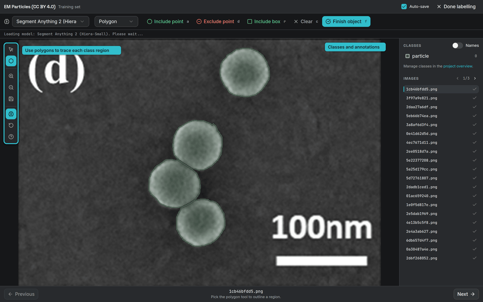
If your dataset has no annotations, use the built-in labeller:

Click Start labelling on the dataset split.
Use the polygon tool to trace a class region.
Choose the appropriate class when you finish the polygon.
Repeat until every relevant region is labelled.

Labelling tips:

Zoom in for fine-grained labeling
Be consistent in your labeling approach (rules for foreground, background)
Use keyboard shortcuts to speed up labeling

For larger datasets, use auto-labelling to propose a mask, then correct it rather than tracing every edge from scratch.

Labeling

Step 3: Model Training

Training Configuration:

Go to the Training tab
Click Start training
Configure the following hyperparameters:
- Model variant: Deeplabv3-Lightweight, Deeplabv3-Medium or Deeplabv3-Large
- Starting weights: Default starts from the pretrained weights that ship with AnyLearning; pick an earlier model of yours to continue training from it
- Learning rate: how far the model moves at each step (0.001 is a sensible start)
- Batch size: how many images are processed together (4 or 8). It must not exceed the number of images in a split, or the run trains on nothing
- Epochs: how many times the model sees the whole training set
- Image size: leave at Model default unless your objects are small, when a larger size helps and costs speed
- Hardware: Automatic uses the GPU when there is one. Choose CPU to leave the GPU free
- Augmentation: flips, rotation and colour jitter, generating variations of your images so the model sees more than it was given
Every setting has an ⓘ beside it that explains it in place.
Click Start training in the dialog to begin

Create a new training

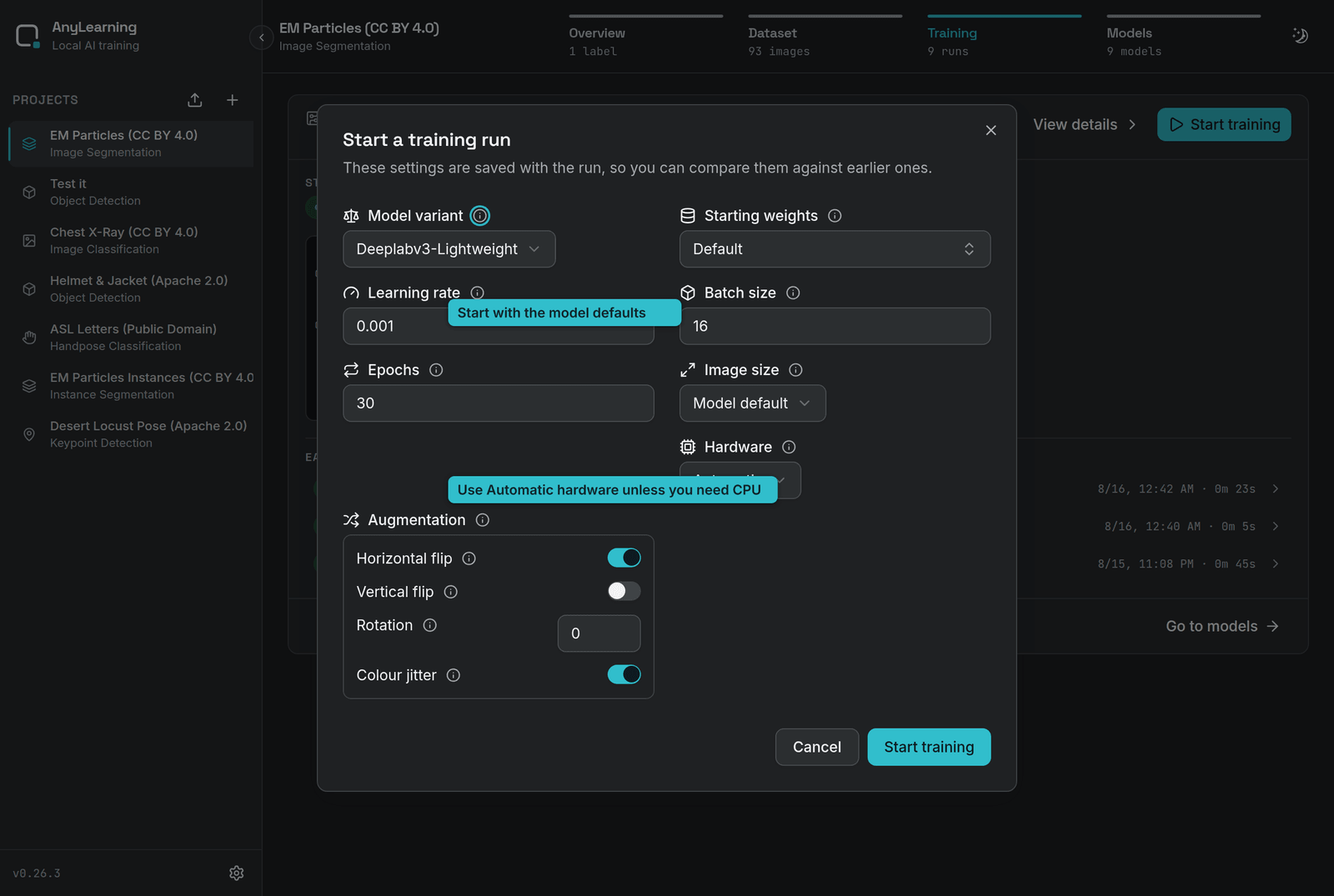
Monitor Training Progress:

View all training sessions in the Training tab.
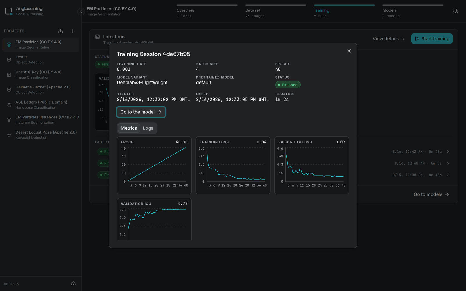
Click View details on a run to inspect its metrics and logs.

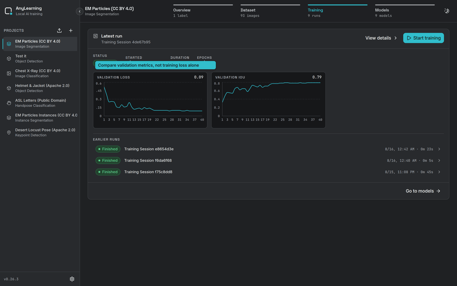
Completed image-segmentation runs

Training Metrics and Logs:

Monitor loss values (segmentation loss)
✅ Check IoU (Intersection over Union) metrics
View training logs for detailed progress information
Watch for signs of overfitting (validation loss getting worse)

Image-segmentation loss and validation metrics

Step 4: Test the Trained Model

After training completes, validate your model's performance:

Go to the Models tab
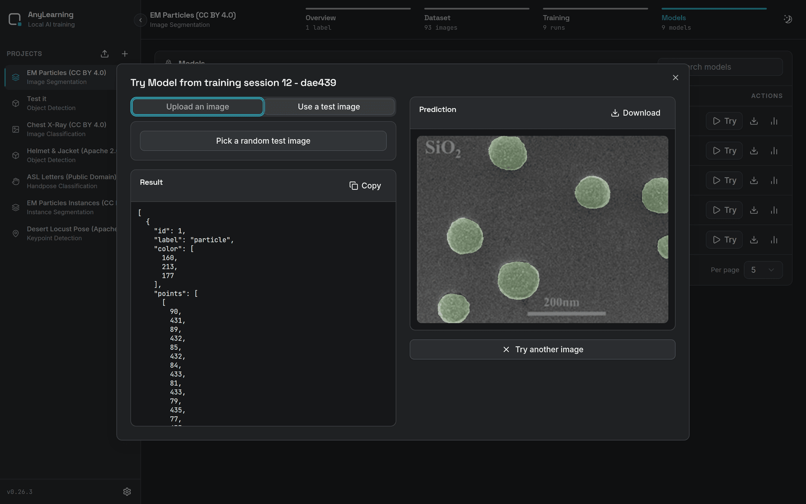
Click Try on the model you want to check.
Choose Use a test image, or upload an image the model has never seen.
Inspect both the overlay and the structured result.

Go to model

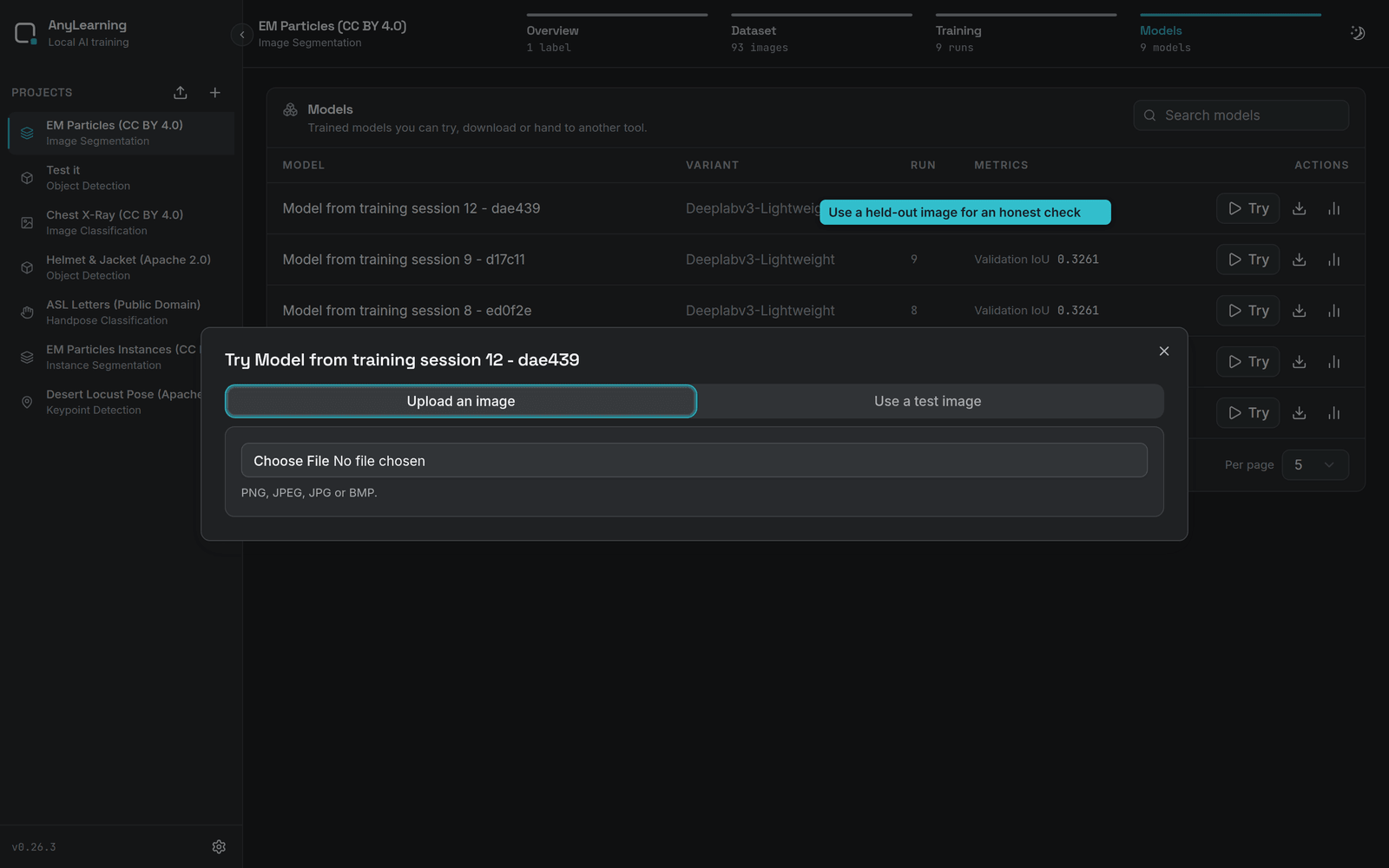
The model will display predictions as segmentation masks overlaid on the input images, highlighting each class with a distinct color.

Segmentation masks overlaid on a held-out image

Step 5: Export the model and use with your code

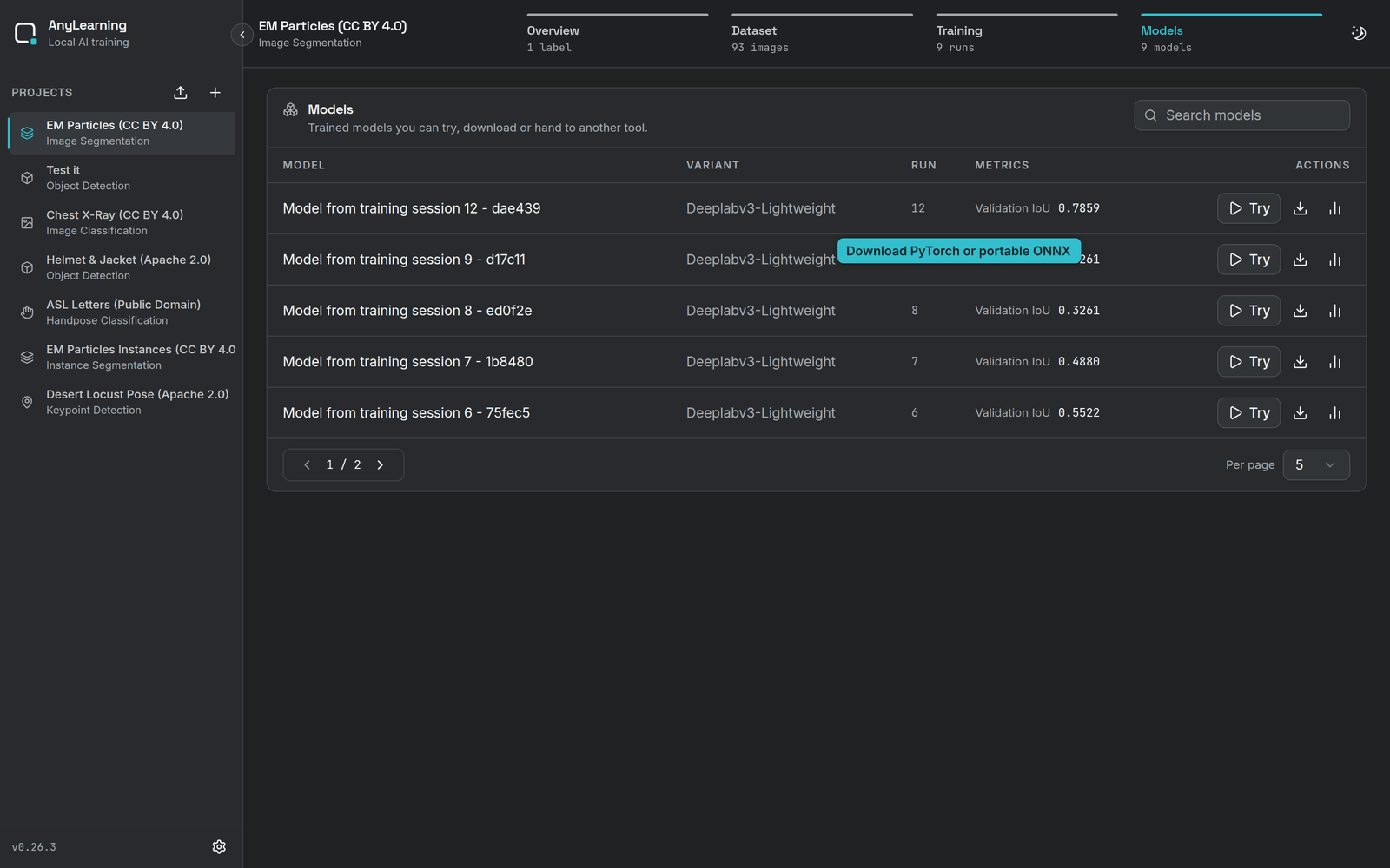
Use the download button on the model's row and pick Raw Model for the PyTorch checkpoint, or ONNX Model for the exported graph. The ONNX download arrives as a zip holding the .onnx file and the config.yml the run was trained with -- unzip it before using the code below.

The inference code is shown below.

Downloading a raw or ONNX segmentation model

5.1. Raw (PyTorch) model usage

Install the necessary libraries:

pip install numpy torch torchvision Pillow opencv-python pyyaml

Run the code:

import yaml
import json
 
import cv2
import numpy as np
from PIL import Image
import torch
from torchvision import transforms
 
CONFIG_PATH = "/path/to/config.yml"
MODEL_PATH = "/path/to/model.pth"
IMAGE_PATH = "/path/to/image.png"
 
 
with open(CONFIG_PATH, "r") as f:
    config = yaml.safe_load(f)
 
def hex_to_rgb(hex_color: str) -> tuple:
    hex_color = hex_color.lstrip('#')
    return tuple(int(hex_color[i:i+2], 16) for i in range(0, len(hex_color), 2))
 
def get_transformations(img_size, mean, std):
    transform = transforms.Compose(
        [
            transforms.Resize((img_size, img_size)),
            transforms.ToTensor(),
            transforms.Normalize(mean, std),
        ]
    )
    return transform
 
label_set = config["data"]["label_set"]
label_id_to_name = {v["id"]: v["name"] for v in label_set}
label_id_to_color = {v["id"]: hex_to_rgb(v["color"]) for v in label_set}
 
model = torch.load(MODEL_PATH)
model.eval()
transform = get_transformations(config["data"]["img_size"],
                                mean=config["data"]["normalize"]["mean"],
                                std=config["data"]["normalize"]["std"])
 
pil_image = Image.open(IMAGE_PATH).convert('RGB')
inp = transform(pil_image)
inp = inp.unsqueeze(0)
 
with torch.no_grad():
    pred_mask = model(inp)
    pred_mask = torch.argmax(pred_mask, dim=1)[0]
 
# Visualize
np_image = np.array(pil_image)
pred_mask = pred_mask.cpu().numpy()
pred_mask = pred_mask.astype(np.uint8)
pred_mask = cv2.resize(pred_mask, (np_image.shape[1], np_image.shape[0]),
                        interpolation=cv2.INTER_NEAREST)
 
visualization_image = np.zeros_like(np_image)
for label_id, color in label_id_to_color.items():
    visualization_image[pred_mask == label_id] = color
 
# Blend with original image
alpha = 0.5
visualization_image = cv2.addWeighted(
    np_image, alpha, visualization_image, 1-alpha, 0
)
 
# save the visualization image
cv2.imwrite("visualization.png", visualization_image)
 
# formatted predictions, to polygon format
formatted_predictions = []
for label_id, name in label_id_to_name.items():
    mask = (pred_mask == label_id).astype(np.uint8)
    contours, _ = cv2.findContours(mask, cv2.RETR_EXTERNAL, cv2.CHAIN_APPROX_SIMPLE)
    all_polygons = []
    for contour in contours:
        if cv2.contourArea(contour) > 5: # filter out small polygons (noise)
            all_polygons.append(contour.flatten().tolist())
    if all_polygons:
        formatted_predictions.append({
            "id": label_id,
            "label": name,
            "color": label_id_to_color[label_id],
            "points": all_polygons,
            "type": "polygon"
        })
 
# save the formatted predictions
with open("formatted_predictions.json", "w") as f:
    json.dump(formatted_predictions, f)

5.2. Exported (ONNX) model usage

Install the necessary libraries:

pip install numpy torch torchvision onnxruntime Pillow opencv-python pyyaml

Run the code:

import yaml
import json
import onnxruntime
import cv2
import numpy as np
from PIL import Image
from torchvision import transforms
 
CONFIG_PATH = "/path/to/config.yml"
MODEL_PATH = "/path/to/model.onnx"
IMAGE_PATH = "/path/to/image.png"
 
with open(CONFIG_PATH, "r") as f:
    config = yaml.safe_load(f)
 
def hex_to_rgb(hex_color: str) -> tuple:
    hex_color = hex_color.lstrip('#')
    return tuple(int(hex_color[i:i+2], 16) for i in range(0, len(hex_color), 2))
 
def get_transformations(img_size, mean, std):
    transform = transforms.Compose(
        [
            transforms.Resize((img_size, img_size)),
            transforms.ToTensor(),
            transforms.Normalize(mean, std),
        ]
    )
    return transform
 
label_set = config["data"]["label_set"]
label_id_to_name = {v["id"]: v["name"] for v in label_set}
label_id_to_color = {v["id"]: hex_to_rgb(v["color"]) for v in label_set}
 
# Initialize ONNX Runtime session
session = onnxruntime.InferenceSession(MODEL_PATH)
input_name = session.get_inputs()[0].name
 
transform = get_transformations(config["data"]["img_size"],
                              mean=config["data"]["normalize"]["mean"],
                              std=config["data"]["normalize"]["std"])
 
pil_image = Image.open(IMAGE_PATH).convert('RGB')
inp = transform(pil_image)
inp = inp.unsqueeze(0).numpy()  # Convert to numpy array for ONNX Runtime
 
# Run inference with ONNX Runtime
pred_mask = session.run(None, {input_name: inp})[0]
pred_mask = np.argmax(pred_mask, axis=1)[0]
 
# Visualize
np_image = np.array(pil_image)
pred_mask = pred_mask.astype(np.uint8)
pred_mask = cv2.resize(pred_mask, (np_image.shape[1], np_image.shape[0]),
                      interpolation=cv2.INTER_NEAREST)
 
visualization_image = np.zeros_like(np_image)
for label_id, color in label_id_to_color.items():
    visualization_image[pred_mask == label_id] = color
 
# Blend with original image
alpha = 0.5
visualization_image = cv2.addWeighted(
    np_image, alpha, visualization_image, 1-alpha, 0
)
 
# save the visualization image
cv2.imwrite("visualization.png", visualization_image)
 
# formatted predictions, to polygon format
formatted_predictions = []
for label_id, name in label_id_to_name.items():
    mask = (pred_mask == label_id).astype(np.uint8)
    contours, _ = cv2.findContours(mask, cv2.RETR_EXTERNAL, cv2.CHAIN_APPROX_SIMPLE)
    all_polygons = []
    for contour in contours:
        if cv2.contourArea(contour) > 5:  # filter out small polygons (noise)
            all_polygons.append(contour.flatten().tolist())
    if all_polygons:
        formatted_predictions.append({
            "id": label_id,
            "label": name,
            "color": label_id_to_color[label_id],
            "points": all_polygons,
            "type": "polygon"
        })
 
# save the formatted predictions
with open("formatted_predictions.json", "w") as f:
    json.dump(formatted_predictions, f)

4. Handpose Classification 6. Instance Segmentation