Instance Segmentation Guide

This guide walks you through creating and training an instance segmentation model using AnyLearning. Instance segmentation outlines each object separately, rather than colouring every pixel of a class the same way.

That difference is the whole reason to choose it. A bounding box cannot separate two objects that overlap, and an image-segmentation mask cannot tell two touching objects apart. Both give you one region where there are two things. Instance segmentation gives every object its own outline, which is what counting anything stacked, packed or crowded actually requires: cells in a micrograph, parcels on a belt, fruit in a crate.

AnyLearning trains Mask R-CNN for this task, with a ResNet-50 or ResNet-101 backbone.

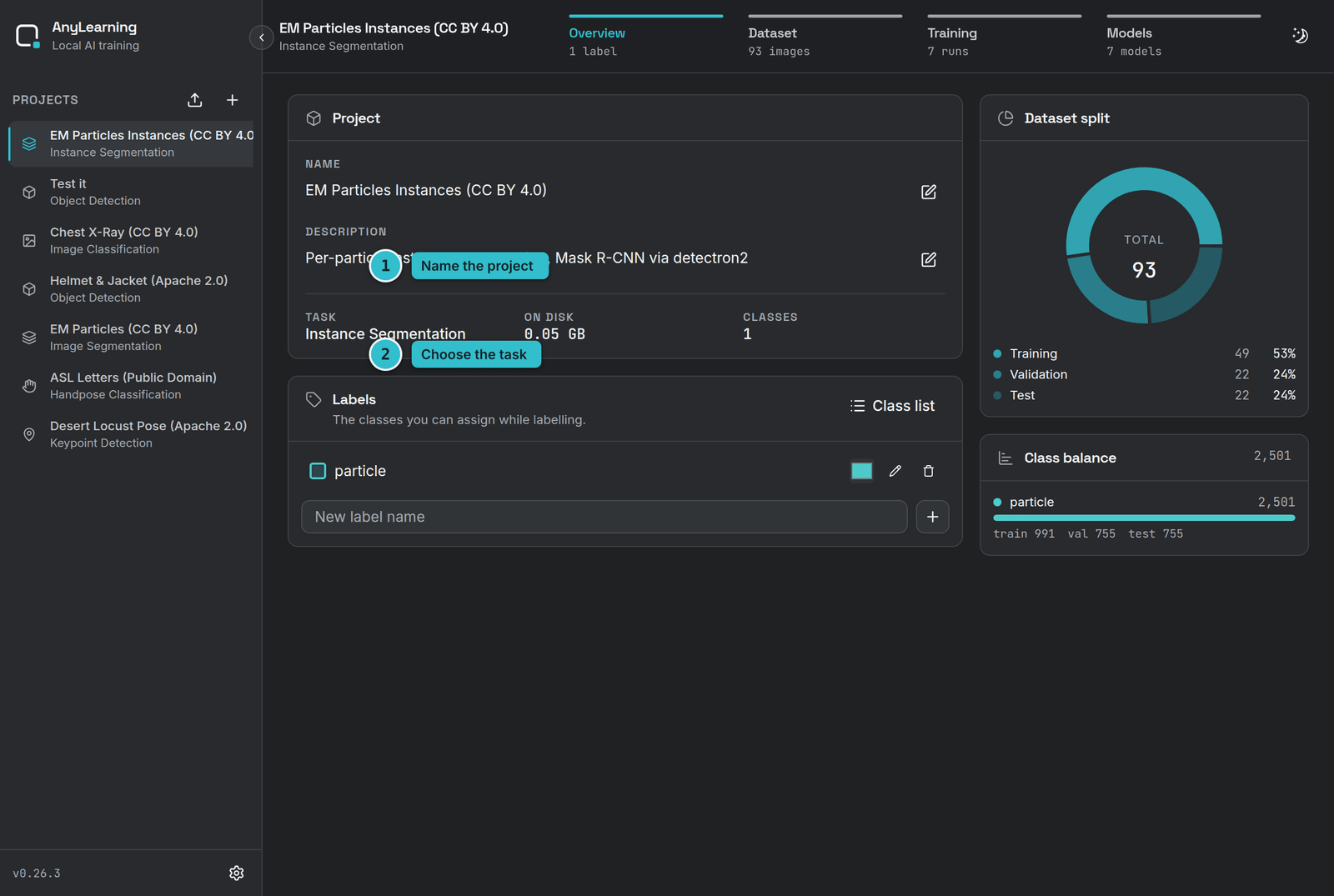
Step 1: Create a Project

1. Click Create project
2. Pick Instance Segmentation as the task
3. Give your project a meaningful name and description

Step 2: Data Preparation

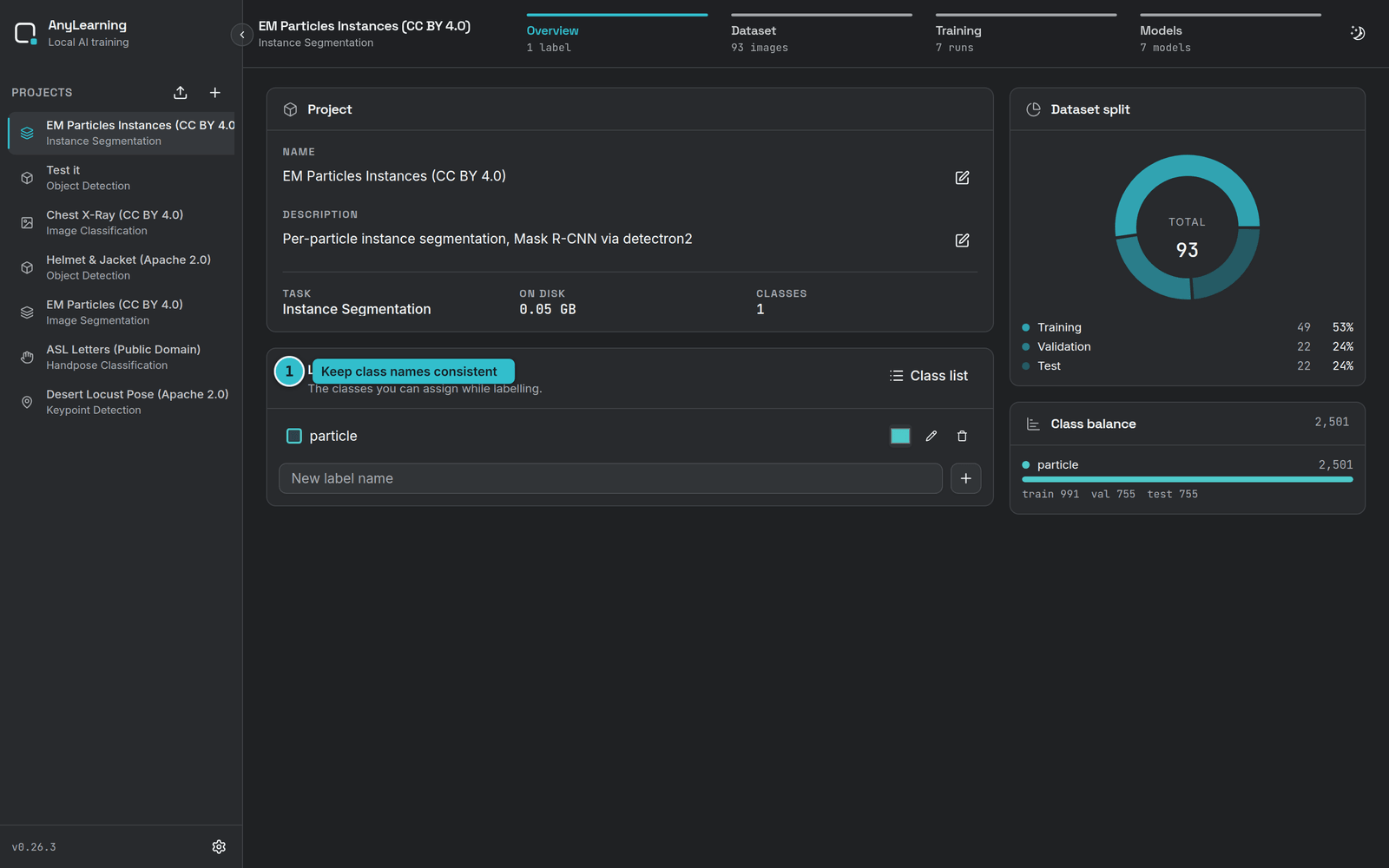
2.1. Create the Label Set

The label set defines the object classes the model will outline. For a particle-counting project one class named particle is enough; for a parcel sorter you might have box and envelope.

To create your label set:

1. Navigate to the Overview tab
2. Enter each class name in the input field
3. Click + after each class name

2.2. Upload the Datasets

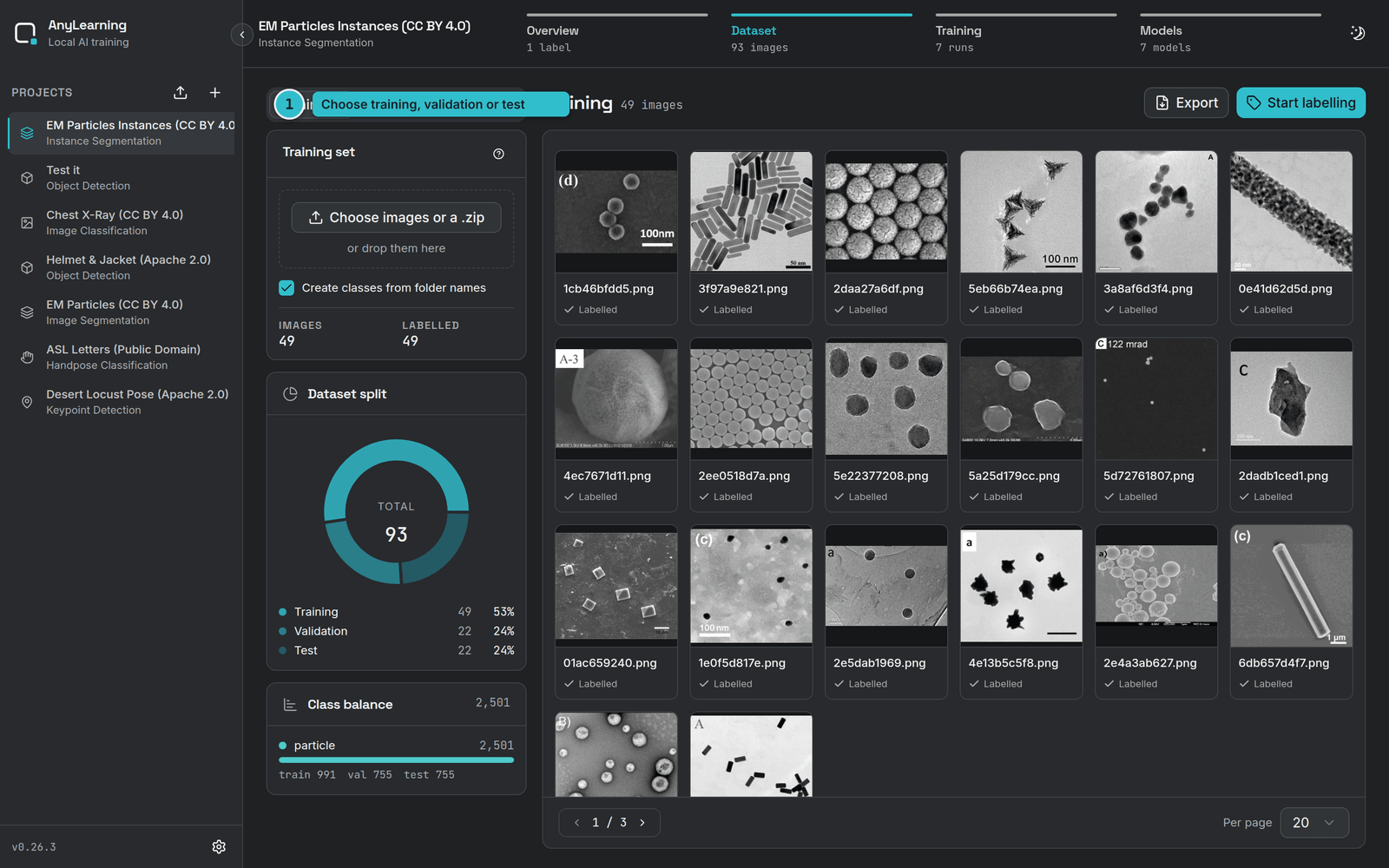
Split your data into three sets:

• Training set: the largest portion (typically 70-80%), used to train
• Validation set: 10-15%, used to watch for overfitting while training
• Test set: 10-15%, kept back to judge the finished model

Upload Process:

1. Go to the Dataset tab and choose the Training, Validation or Test set.
2. Click Choose images or a .zip, or drop files straight onto the panel. Several images at once is fine, and so is one .zip per split.
3. If your images are already annotated, upload the archive as it is: COCO, YOLO, LabelMe and AnyLabeling are all read, and the annotations come in with the images. Ticking Create classes from folder names takes the class list from the archive rather than needing step 2.1 first.
4. Wait for the upload to finish. The image and label counts under the panel update as it goes.

Important: instance segmentation learns from polygons, one per object. An archive whose annotations are rectangles will import, but the model will only ever learn box-shaped objects.

2.3. Label the Data

1. Click Start labelling on the split you want to annotate.
2. Pick the polygon tool and click around one object at a time. Each object gets its own polygon, even where two of them touch — that separation is exactly what this model type learns.
3. Choose the class for each shape as you finish it.
4. Annotations save as you go; Done labelling returns to the dataset.

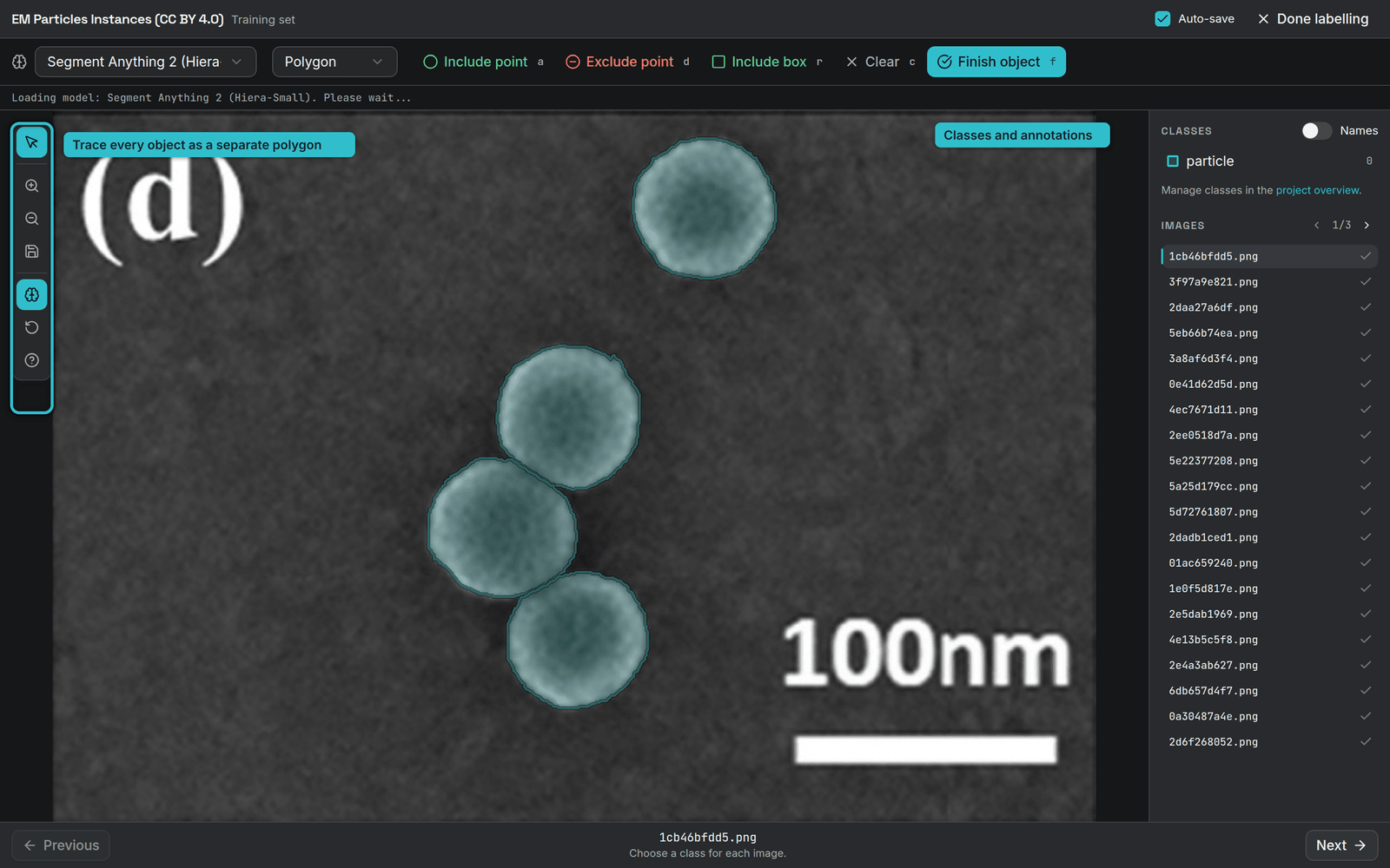
Auto-labelling helps here more than anywhere else: Segment Anything outlines a single object from one click, which is a great deal faster than tracing a particle by hand. See the auto labeling guide.

Step 3: Model Training

Training Configuration:

1. Go to the Training tab

2. Click Start training

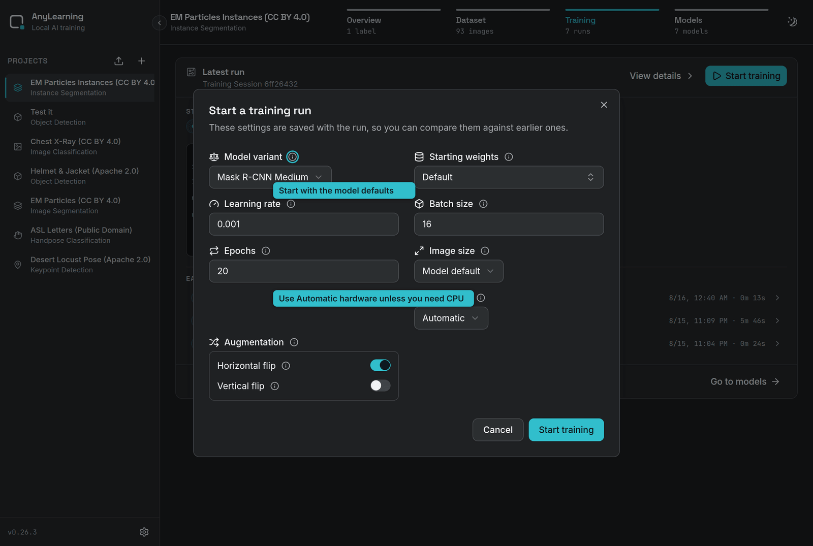
3. Configure the following hyperparameters:

   • Model variant: Mask R-CNN Medium (ResNet-50) or Mask R-CNN Large (ResNet-101)
   • Starting weights: Default starts from the COCO-pretrained weights that ship with AnyLearning; pick an earlier model of yours to continue training from it
   • Learning rate: how far the model moves at each step (0.001 is a sensible start)
   • Batch size: how many images are processed together (2 or 4; Mask R-CNN uses far more memory per image than the other model types). It must not exceed the number of images in a split, or the run trains on nothing
   • Epochs: how many times the model sees the whole training set
   • Image size: leave at Model default unless your objects are small, when a larger size helps and costs speed
   • Hardware: Automatic uses the GPU when there is one. Choose CPU to leave the GPU free
   • Augmentation: flips and rotation, generating variations of your images so the model sees more than it was given

   Every setting has an ⓘ beside it that explains it in place.

4. Click Start training in the dialog to begin

Monitor Training Progress:

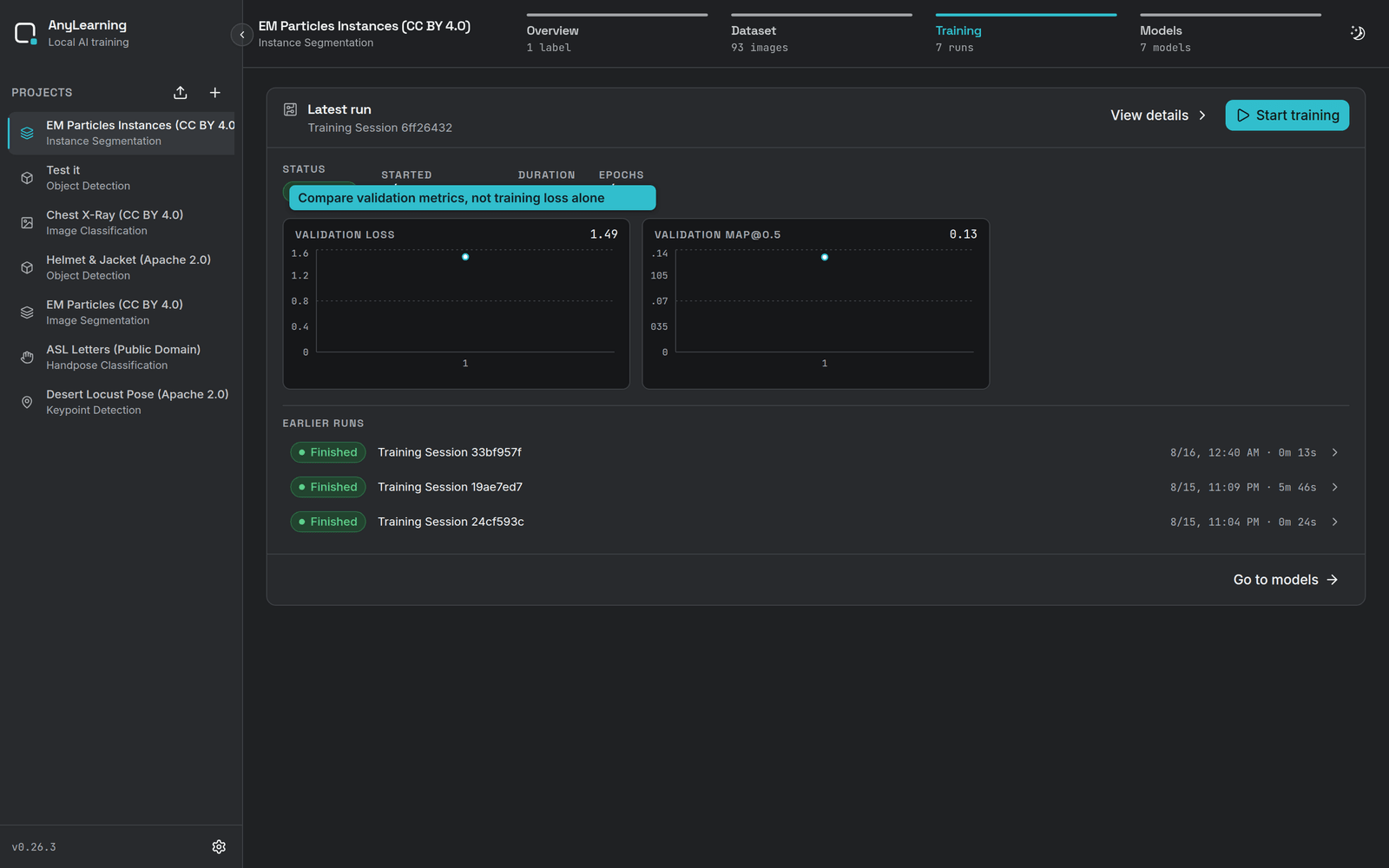
• View all training runs in the Training tab
• Click View details on any run to see its metrics and logs

Training Metrics and Logs:

Instance segmentation reports two mAP figures beside the losses:

• Validation mAP@0.5: how well the model finds objects at a lenient overlap
• Validation mAP@0.5:0.95: the stricter average, which is the one to compare runs on

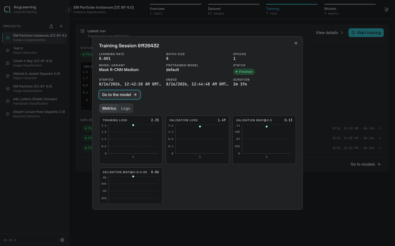
Both rise as the model improves. Losses that fall while mAP stalls usually mean the model is memorising the training set.

Step 4: Test the Trained Model

After training completes, check what the model actually does:

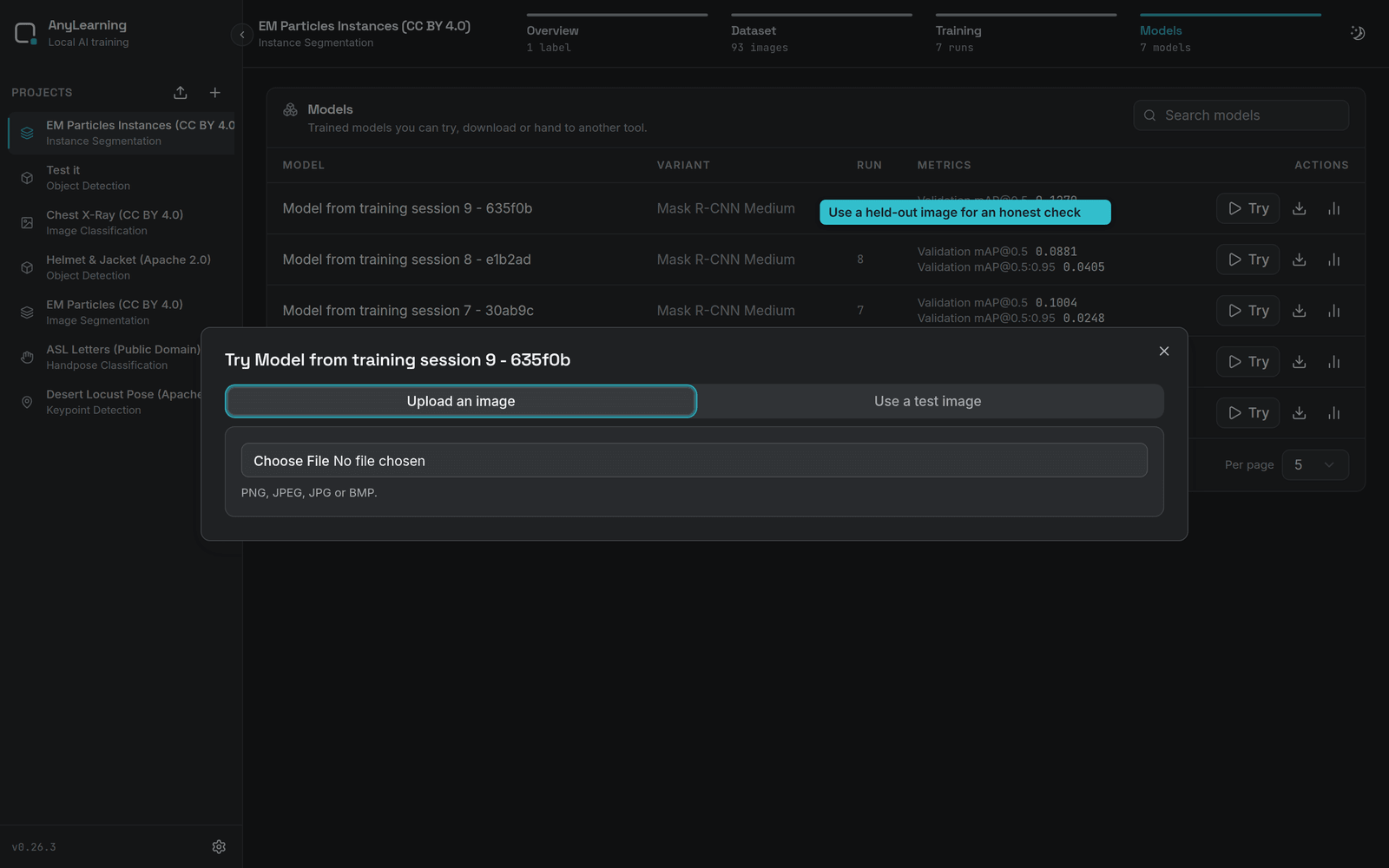
1. Go to the Models tab
2. Click Try on the model you want to check
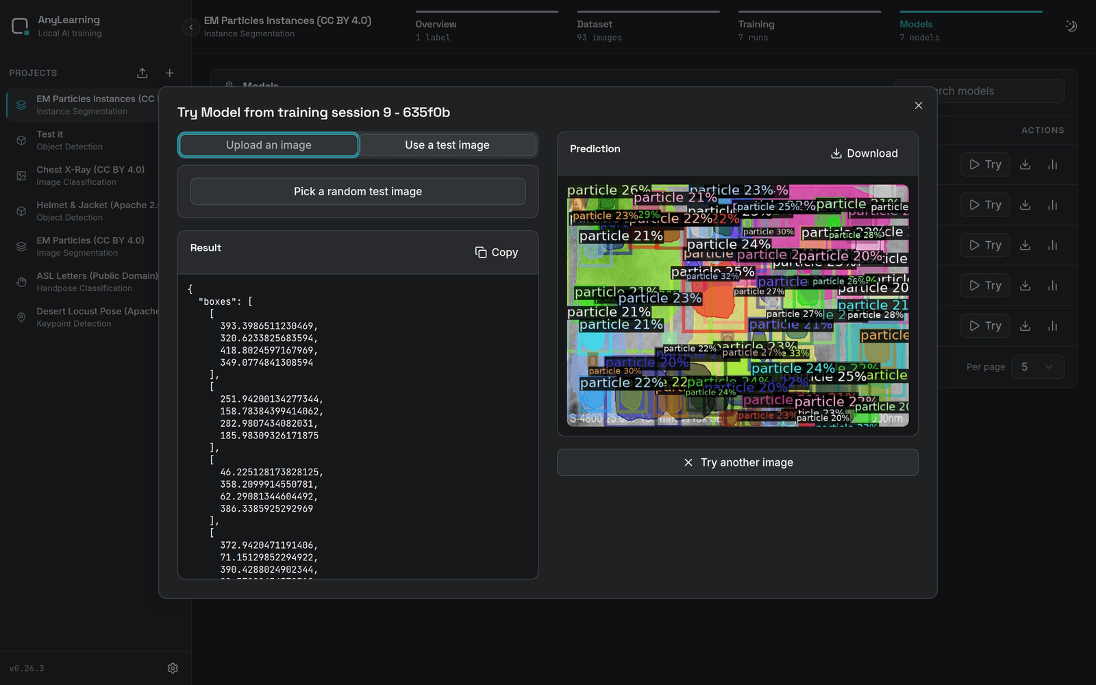
3. Choose Use a test image to take one from your test split, or Upload an image for a picture the model has never seen
4. Each detected object comes back with its own outline, class and confidence

Step 5: Export the model and use with your code

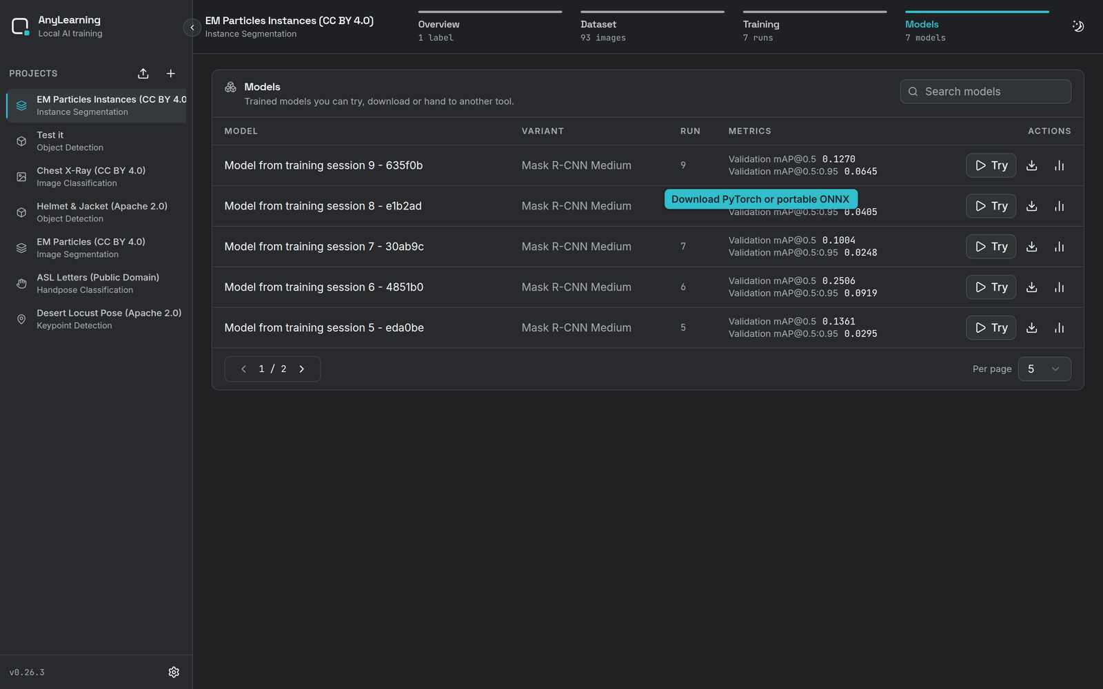
Use the download button on the model's row and pick Raw Model for the PyTorch checkpoint, or ONNX Model for the exported graph. The ONNX download arrives as a zip holding the .onnx file and the config.yml the run was trained with. Unzip it before using the code below.

5.1. Raw (PyTorch) model usage

The checkpoint is a whole pickled Mask R-CNN, so detectron2 has to be installed to load it:

pip install torch torchvision opencv-python pyyaml
pip install "git+https://github.com/facebookresearch/detectron2.git"

• Run the code:

import cv2
import torch
import yaml
 
MODEL_PATH = "best_model.pth"      # Raw (PyTorch) model file
CONFIG_PATH = "config.yml"         # From the ONNX download
IMAGE_PATH = "test_image.png"
 
config = yaml.safe_load(open(CONFIG_PATH))
# The class list lives under data.label_set, in the order the model predicts.
class_names = [label["name"] for label in config["data"]["label_set"]]
 
# A whole pickled module, so detectron2 must be importable to unpickle it.
# weights_only=False is required from torch 2.6 onwards.
model = torch.load(MODEL_PATH, map_location="cpu", weights_only=False)
model.eval()
 
image = cv2.imread(IMAGE_PATH)     # BGR, which is what the model was trained on
height, width = image.shape[:2]
tensor = torch.as_tensor(image.astype("float32").transpose(2, 0, 1))
 
with torch.no_grad():
    outputs = model([{"image": tensor, "height": height, "width": width}])[0]
 
instances = outputs["instances"].to("cpu")
print(f"{len(instances)} objects found")
 
for index in range(len(instances)):
    label = class_names[int(instances.pred_classes[index])]
    score = float(instances.scores[index])
    box = [round(v, 1) for v in instances.pred_boxes.tensor[index].tolist()]
 
    # The mask is a full-size boolean image; contours turn it into a polygon.
    mask = instances.pred_masks[index].numpy().astype("uint8")
    contours, _ = cv2.findContours(mask, cv2.RETR_EXTERNAL, cv2.CHAIN_APPROX_SIMPLE)
    polygon = [point.flatten().tolist() for point in contours]
 
    print(f"{label} {score:.2f} box={box} area={int(mask.sum())}px")

Output looks like this, one line per object, each with its own mask:

77 objects found
particle 0.98 box=[389.4, 125.7, 595.4, 314.4] area=17340px
particle 0.97 box=[599.3, 300.3, 696.0, 446.1] area=8718px
particle 0.95 box=[485.7, 454.8, 528.4, 501.0] area=950px

Counting objects is then len(instances), and filtering by confidence is a comparison on instances.scores.

5.2. A note on the ONNX export

The ONNX graph is exported with detectron2's tracing adapter and without post-processing, so its outputs are in the model's internal resolution and need the same resizing and mask-pasting steps detectron2 does internally. If you want predictions in image coordinates with the least work, use the raw checkpoint above; the ONNX file is there for runtimes that cannot load PyTorch at all.